Preprocessing Transforms Gallery

In PathML, preprocessing pipelines are created by composing modular Transforms.

The following tutorial contains an overview of the PathML pre-processing Transforms, with examples.

We will divide Transforms into three primary categories, depending on their function:

1. Transforms that modify an image

   • Gaussian Blur

   • Median Blur

   • Box Blur

   • Stain Normalization

   • Superpixel Interpolation

2. Transforms that create a mask

   • Nucleus Detection

   • Binary Threshold

3. Transforms that modify a mask

   • Morphological Closing

   • Morphological Opening

   • Foreground Detection

   • Tissue Detection

import matplotlib.pyplot as plt
import copy

from pathml.core import HESlide, Tile, types
from pathml.utils import plot_mask, RGB_to_GREY
from pathml.preprocessing import (
    BoxBlur, GaussianBlur, MedianBlur,
    NucleusDetectionHE, StainNormalizationHE, SuperpixelInterpolation,
    ForegroundDetection, TissueDetectionHE, BinaryThreshold,
    MorphClose, MorphOpen
)

fontsize = 14

Note that a Transform operates on Tile objects. We must first load a whole-slide image, extract a smaller region, and create a Tile:

wsi = HESlide("./../data/CMU-1-Small-Region.svs")
region = wsi.slide.extract_region(location = (900, 800), size = (500, 500))

def smalltile():
    # convenience function to create a new tile
    return Tile(region, coords = (0, 0), name = "testregion", slide_type = types.HE)

Transforms that modify an image

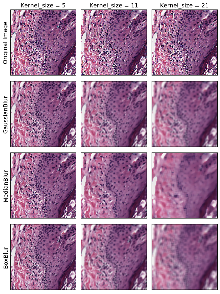
Blurring Transforms

We’ll start with the 3 blurring transforms: GaussianBlur, MedianBlur, and BoxBlur

Blurriness can be control with the kernel_size parameter. A larger kernel width yields a more blurred result for all blurring transforms:

blurs = ["Original Image", GaussianBlur, MedianBlur, BoxBlur]
blur_name = ["Original Image", "GaussianBlur", "MedianBlur", "BoxBlur"]
k_size = [5, 11, 21]
fig, axarr = plt.subplots(nrows=4, ncols=3, figsize=(7.5, 10))
for i, blur in enumerate(blurs):
    for j, kernel_size in enumerate(k_size):
        tile = smalltile()
        if blur != "Original Image":
            b = blur(kernel_size = kernel_size)
            b.apply(tile)
        ax = axarr[i, j]
        ax.imshow(tile.image)
        if i == 0:
            ax.set_title(f"Kernel_size = {kernel_size}", fontsize=fontsize)
        if j == 0:
            ax.set_ylabel(blur_name[i], fontsize = fontsize)
for a in axarr.ravel():
    a.set_xticks([])
    a.set_yticks([])
plt.tight_layout()
plt.show()

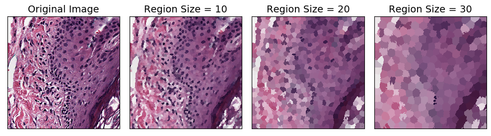
Superpixel Interpolation

Superpixel interpolation is a method for grouping together nearby similar pixels to form larger “superpixels.” The SuperpixelInterpolation Transform divides the input image into superpixels using SLIC algorithm, then interpolates each superpixel with average color. The region_size parameter controls how big the superpixels are:

region_sizes = ["original", 10, 20, 30]
fig, axarr = plt.subplots(nrows=1, ncols=4, figsize=(10, 10))
for i, region_size in enumerate(region_sizes):
    tile = smalltile()
    if region_size == "original":
        axarr[i].set_title("Original Image", fontsize = fontsize)
    else:
        t = SuperpixelInterpolation(region_size = region_size)
        t.apply(tile)
        axarr[i].set_title(f"Region Size = {region_size}", fontsize = fontsize)
    axarr[i].imshow(tile.image)
for ax in axarr.ravel():
    ax.set_yticks([])
    ax.set_xticks([])
plt.tight_layout()
plt.show()

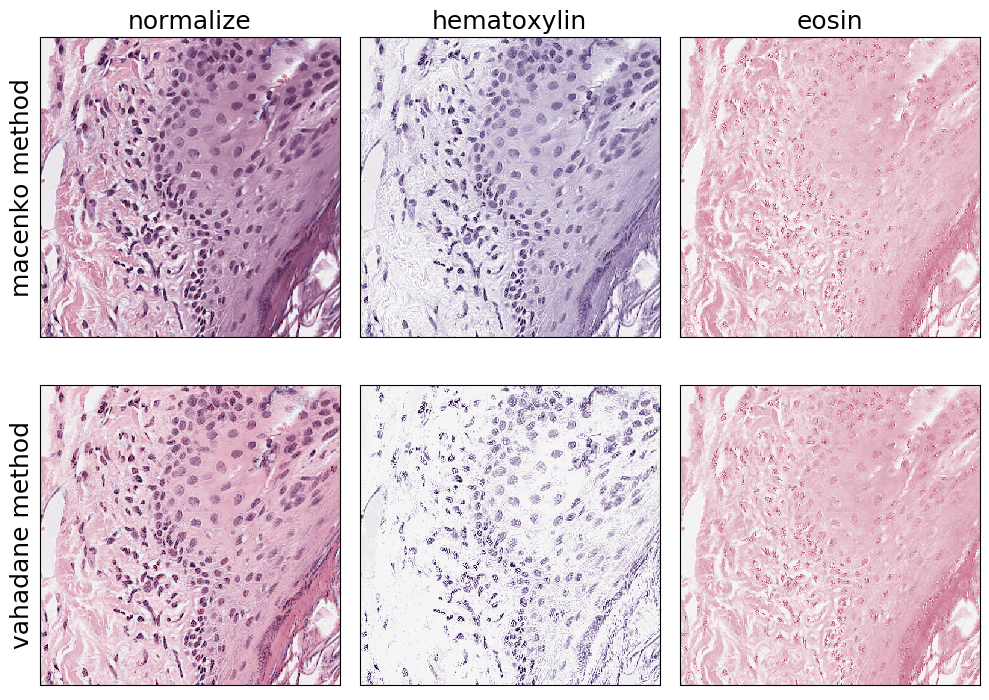
Stain Normalization

H&E images are a combination of two stains: hematoxylin and eosin. Stain deconvolution methods attempt to estimate the relative contribution of each stain for each pixel. Each stain can then be pulled out into a separate image, and the deconvolved images can then be recombined to normalize the appearance of the image.

The StainNormalizationHE Transform implements two algorithms for stain deconvolution.

fig, axarr = plt.subplots(nrows=2, ncols=3, figsize=(10, 7.5))
fontsize = 18
for i, method in enumerate(["macenko", "vahadane"]):
    for j, target in enumerate(["normalize", "hematoxylin", "eosin"]):
        tile = smalltile()
        normalizer = StainNormalizationHE(target = target, stain_estimation_method = method)
        normalizer.apply(tile)
        ax = axarr[i, j]
        ax.imshow(tile.image)
        if j == 0:
            ax.set_ylabel(f"{method} method", fontsize=fontsize)
        if i == 0:
            ax.set_title(target, fontsize = fontsize)
for a in axarr.ravel():
    a.set_xticks([])
    a.set_yticks([])
plt.tight_layout()
plt.show()

Transforms that create a mask

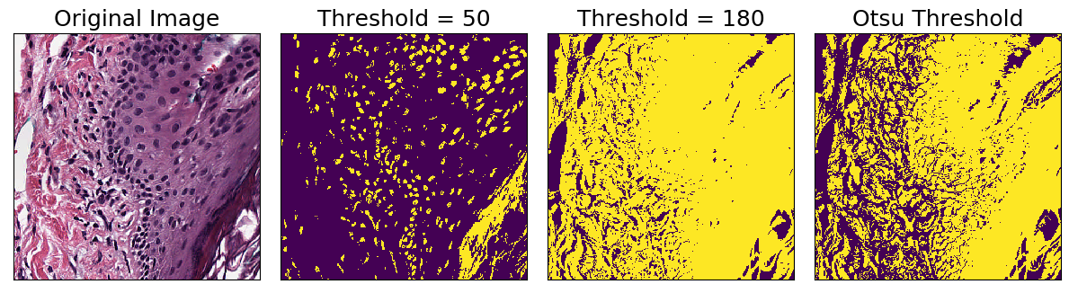
Binary Threshold

The BinaryThreshold transform creates a mask by classifying whether each pixel is above or below the given threshold. Note that you can supply a threshold parameter, or use Otsu’s method to automatically determine a threshold:

thresholds = ["original", 50, 180, "otsu"]
fig, axarr = plt.subplots(nrows=1, ncols=len(thresholds), figsize=(12, 6))
for i, thresh in enumerate(thresholds):
    tile = smalltile()
    if thresh == "original":
        axarr[i].set_title("Original Image", fontsize = fontsize)
        axarr[i].imshow(tile.image)
    elif thresh == "otsu":
        t = BinaryThreshold(mask_name = "binary_threshold",
                            inverse = True, use_otsu = True)
        t.apply(tile)
        axarr[i].set_title(f"Otsu Threshold", fontsize = fontsize)
        axarr[i].imshow(tile.masks["binary_threshold"])
    else:
        t = BinaryThreshold(mask_name = "binary_threshold", threshold = thresh,
                            inverse = True, use_otsu = False)
        t.apply(tile)
        axarr[i].set_title(f"Threshold = {thresh}", fontsize = fontsize)
        axarr[i].imshow(tile.masks["binary_threshold"])
for ax in axarr.ravel():
    ax.set_yticks([])
    ax.set_xticks([])
plt.tight_layout()
plt.show()

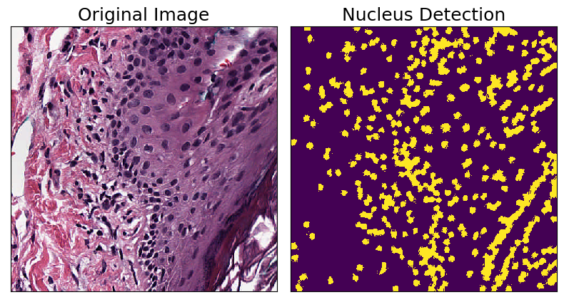
Nucleus Detection

The NucleusDetectionHE transform employs a simple nucleus detection algorithm for H&E stained images. It works by first separating hematoxylin channel, then doing interpolation using superpixels, and finally using Otsu’s method for binary thresholding. This is an example of a compound Transform created by combining several other Transforms:

tile = smalltile()
nucleus_detection = NucleusDetectionHE(mask_name = "detect_nuclei")
nucleus_detection.apply(tile)

fig, axarr = plt.subplots(nrows=1, ncols=2, figsize=(8, 8))
axarr[0].imshow(tile.image)
axarr[0].set_title("Original Image", fontsize=fontsize)
axarr[1].imshow(tile.masks["detect_nuclei"])
axarr[1].set_title("Nucleus Detection", fontsize=fontsize)
for ax in axarr.ravel():
    ax.set_yticks([])
    ax.set_xticks([])
plt.tight_layout()
plt.show()

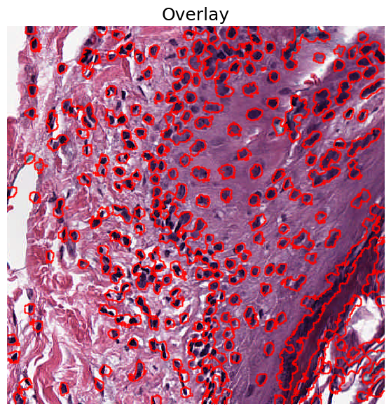
We can also overlay the results on the original image to see which regions were identified as being nuclei:

fig, ax = plt.subplots(figsize=(7, 7))
plot_mask(im = tile.image, mask_in=tile.masks["detect_nuclei"], ax = ax)
plt.title("Overlay", fontsize = fontsize)
plt.axis('off')
plt.show()

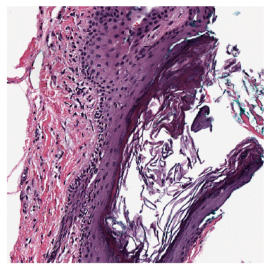
Transforms that modify a mask

For the following transforms, we’ll use a Tile containing a larger region extracted from the slide.

bigregion = wsi.slide.extract_region(location = (800, 800), size = (1000, 1000))

def bigtile():
    # convenience function to create a new tile with a binary mask
    bigtile = Tile(bigregion, coords = (0, 0), name = "testregion", slide_type = types.HE)
    BinaryThreshold(mask_name = "binary_threshold", inverse=True,
                    threshold = 100, use_otsu = False).apply(bigtile)
    return bigtile

plt.imshow(bigregion)
plt.axis("off")
plt.show()

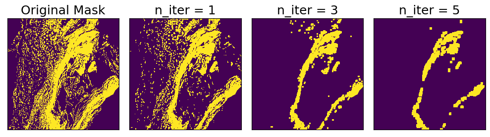
Morphological Opening

Morphological opening reduces noise in a binary mask by first applying binary erosion n times, and then applying binary dilation n times. The effect is to remove small objects from the background. The strength of the effect can be controlled by setting n

ns = ["Original Mask", 1, 3, 5]
fig, axarr = plt.subplots(nrows=1, ncols=4, figsize=(10, 10))
for i, n in enumerate(ns):
    tile = bigtile()
    if n == "Original Mask":
        axarr[i].set_title("Original Mask", fontsize = fontsize)
    else:
        t = MorphOpen(mask_name = "binary_threshold", n_iterations=n)
        t.apply(tile)
        axarr[i].set_title(f"n_iter = {n}", fontsize = fontsize)
    axarr[i].imshow(tile.masks["binary_threshold"])
for ax in axarr.ravel():
    ax.set_yticks([])
    ax.set_xticks([])
plt.tight_layout()
plt.show()

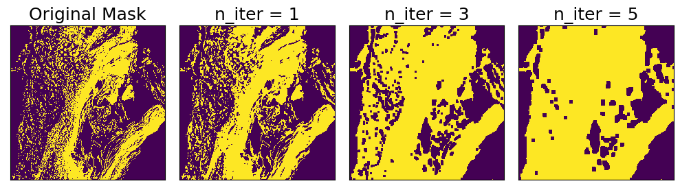
Morphological Closing

Morphological closing is similar to opening, but in the opposite order: first, binary dilation is applied n times, then binary erosion is applied n times. The effect is to reduce noise in a binary mask by closing small holes in the foreground. The strength of the effect can be controlled by setting n

ns = ["Original Mask", 1, 3, 5]
fig, axarr = plt.subplots(nrows=1, ncols=4, figsize=(10, 10))
for i, n in enumerate(ns):
    tile = bigtile()
    if n == "Original Mask":
        axarr[i].set_title("Original Mask", fontsize = fontsize)
    else:
        t = MorphClose(mask_name = "binary_threshold", n_iterations=n)
        t.apply(tile)
        axarr[i].set_title(f"n_iter = {n}", fontsize = fontsize)
    axarr[i].imshow(tile.masks["binary_threshold"])
for ax in axarr.ravel():
    ax.set_yticks([])
    ax.set_xticks([])
plt.tight_layout()
plt.show()

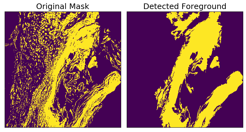
Foreground Detection

This transform operates on binary masks and identifies regions that have a total area greater than specified threshold. Supports including holes within foreground regions, or excluding holes above a specified area threshold.

tile = bigtile()
foreground_detector = ForegroundDetection(mask_name = "binary_threshold")
original_mask = tile.masks["binary_threshold"].copy()
foreground_detector.apply(tile)

fig, axarr = plt.subplots(nrows=1, ncols=2, figsize=(8, 8))
axarr[0].imshow(original_mask)
axarr[0].set_title("Original Mask", fontsize=fontsize)
axarr[1].imshow(tile.masks["binary_threshold"])
axarr[1].set_title("Detected Foreground", fontsize=fontsize)
for ax in axarr.ravel():
    ax.set_yticks([])
    ax.set_xticks([])
plt.tight_layout()
plt.show()

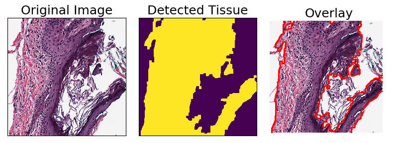
Tissue Detection

TissueDetectionHE is a Transform for detecting regions of tissue from an H&E image. It is composed by applying a sequence of other Transforms: first a median blur, then binary thresholding, then morphological opening and closing, and finally foreground detection.

tile = bigtile()

tissue_detector = TissueDetectionHE(mask_name = "tissue", outer_contours_only=True)
tissue_detector.apply(tile)

fig, axarr = plt.subplots(nrows=1, ncols=3, figsize=(8, 8))
axarr[0].imshow(tile.image)
axarr[0].set_title("Original Image", fontsize=fontsize)
axarr[1].imshow(tile.masks["tissue"])
axarr[1].set_title("Detected Tissue", fontsize=fontsize)
plot_mask(im = tile.image, mask_in=tile.masks["tissue"], ax = axarr[2])
axarr[2].set_title("Overlay", fontsize=fontsize)

for ax in axarr.ravel():
    ax.set_yticks([])
    ax.set_xticks([])
plt.tight_layout()
plt.show()