Multiparametric Imaging: CODEX
In this tutorial, we will analyze the CODEX images provided by Schürch et. al: https://www.ncbi.nlm.nih.gov/pmc/articles/PMC7479520/.
Here, we will use PathML to process a large number of CODEX slides (140 slides) simultaneously through the SlideDataset class. We also show how the generated count matrices can be used to investigate the complex spatial architecture of the iTME in colorectal cancer.
[1]:
from os import listdir, path, getcwd
import glob
import re
import pandas as pd
from pathml.core import SlideDataset
from pathml.core.slide_data import VectraSlide
from pathml.core.slide_data import CODEXSlide
from pathml.preprocessing.pipeline import Pipeline
from pathml.preprocessing.transforms import SegmentMIF, QuantifyMIF, CollapseRunsCODEX
import numpy as np
import matplotlib.pyplot as plt
from matplotlib.pyplot import rc_context
from dask.distributed import Client, LocalCluster
from deepcell.utils.plot_utils import make_outline_overlay
from deepcell.utils.plot_utils import create_rgb_image
import scanpy as sc
import squidpy as sq
import anndata as ad
import bbknn
from joblib import parallel_backend
In /Users/mohamedomar/opt/anaconda3/envs/pathml2/lib/python3.8/site-packages/matplotlib/mpl-data/stylelib/_classic_test.mplstyle:
The text.latex.preview rcparam was deprecated in Matplotlib 3.3 and will be removed two minor releases later.
In /Users/mohamedomar/opt/anaconda3/envs/pathml2/lib/python3.8/site-packages/matplotlib/mpl-data/stylelib/_classic_test.mplstyle:
The mathtext.fallback_to_cm rcparam was deprecated in Matplotlib 3.3 and will be removed two minor releases later.
In /Users/mohamedomar/opt/anaconda3/envs/pathml2/lib/python3.8/site-packages/matplotlib/mpl-data/stylelib/_classic_test.mplstyle: Support for setting the 'mathtext.fallback_to_cm' rcParam is deprecated since 3.3 and will be removed two minor releases later; use 'mathtext.fallback : 'cm' instead.
In /Users/mohamedomar/opt/anaconda3/envs/pathml2/lib/python3.8/site-packages/matplotlib/mpl-data/stylelib/_classic_test.mplstyle:
The validate_bool_maybe_none function was deprecated in Matplotlib 3.3 and will be removed two minor releases later.
In /Users/mohamedomar/opt/anaconda3/envs/pathml2/lib/python3.8/site-packages/matplotlib/mpl-data/stylelib/_classic_test.mplstyle:
The savefig.jpeg_quality rcparam was deprecated in Matplotlib 3.3 and will be removed two minor releases later.
In /Users/mohamedomar/opt/anaconda3/envs/pathml2/lib/python3.8/site-packages/matplotlib/mpl-data/stylelib/_classic_test.mplstyle:
The keymap.all_axes rcparam was deprecated in Matplotlib 3.3 and will be removed two minor releases later.
In /Users/mohamedomar/opt/anaconda3/envs/pathml2/lib/python3.8/site-packages/matplotlib/mpl-data/stylelib/_classic_test.mplstyle:
The animation.avconv_path rcparam was deprecated in Matplotlib 3.3 and will be removed two minor releases later.
In /Users/mohamedomar/opt/anaconda3/envs/pathml2/lib/python3.8/site-packages/matplotlib/mpl-data/stylelib/_classic_test.mplstyle:
The animation.avconv_args rcparam was deprecated in Matplotlib 3.3 and will be removed two minor releases later.
/Users/mohamedomar/opt/anaconda3/envs/pathml2/lib/python3.8/site-packages/tensorflow/python/keras/optimizer_v2/optimizer_v2.py:374: UserWarning: The `lr` argument is deprecated, use `learning_rate` instead.
  warnings.warn(
[2]:
# set working directory
%cd "~/Documents/Research/Projects/CRC_TMA"
/Users/mohamedomar/Documents/Research/Projects/CRC_TMA
[3]:
## Read channel names
channelnames = pd.read_csv(
    "data/channelNames.txt", header=None, dtype=str, low_memory=False
)
channelnames
[3]:
| 0 | |
|---|---|
| 0 | HOECHST1 |
| 1 | blank |
| 2 | blank |
| 3 | blank |
| 4 | HOECHST2 |
| ... | ... |
| 87 | empty-Cy5-22 |
| 88 | HOECHST23 |
| 89 | empty-A488-23 |
| 90 | empty-Cy3-23 |
| 91 | DRAQ5 |
92 rows × 1 columns
Reading the slides
[21]:
dirpath = r"/Volumes/Mohamed/CRC"

# assuming that all slides are in a single directory, all with .tif file extension
for A, B in [listdir(dirpath)]:
    vectra_list_A = [
        CODEXSlide(p, stain="IF") for p in glob.glob(path.join(dirpath, A, "*.tif"))
    ]
    vectra_list_B = [
        CODEXSlide(p, stain="IF") for p in glob.glob(path.join(dirpath, B, "*.tif"))
    ]
    # Fix the slide names and add origin labels (A, B)
    for slide_A, slide_B in zip(vectra_list_A, vectra_list_B):
        slide_A.name = re.sub("X.*", "A", slide_A.name)
        slide_B.name = re.sub("X.*", "B", slide_B.name)
    # Store all slides in a SlideDataSet object
    dataset = SlideDataset(vectra_list_A + vectra_list_B)
Define and run the preprocessing pipeline
[8]:
# Here, we use DAPI (channel 0) and vimentin (channel 29) for segmentation
# Z=0 since we are processing images with a single slice (best focus)
pipe = Pipeline(
    [
        CollapseRunsCODEX(z=0),
        SegmentMIF(
            model="mesmer",
            nuclear_channel=0,
            cytoplasm_channel=29,
            image_resolution=0.377442,
        ),
        QuantifyMIF(segmentation_mask="cell_segmentation"),
    ]
)

# Initialize a dask cluster using 10 workers. PathML pipelines can be run in distributed mode on
# cloud compute or a cluster using dask.distributed.
cluster = LocalCluster(n_workers=10, threads_per_worker=1, processes=True)
client = Client(cluster)

# Run the pipeline
dataset.run(
    pipe, distributed=True, client=client, tile_size=(1920, 1440), tile_pad=False
)

# Write the processed datasets to disk
dataset.write("data/dataset_processed.h5")
Extract and concatenate the resulting count matrices
Combine the count matrices into a single adata object:
[ ]:
##  Combine the count matrices into a single adata object:
adata = ad.concat(
    [x.counts for x in dataset.slides], join="outer", label="Region", index_unique="_"
)
# Fix and replace the regions names
origin = adata.obs["Region"]
origin = origin.astype(str).str.replace("[^a-zA-Z0-9 \n\.]", "")
origin = origin.astype(str).str.replace("[\n]", "")
origin = origin.str.replace("SlideDataname", "")
adata.obs["Region"] = origin

# save the adata object
adata_combined.write(filename="./data/adata_combined.h5ad")
[6]:
# Rename the variable names (channels) in the adata object
adata.var_names = channelnames[0]
adata.var_names_make_unique()
Filter the cells using the DAPI and DRAQ5 intensity
[7]:
# Plot the DAPI intensity distribution:
sc.pl.violin(adata, keys=["HOECHST1", "DRAQ5"], multi_panel=True)
/Users/mohamedomar/opt/anaconda3/envs/pathml2/lib/python3.8/site-packages/anndata/_core/anndata.py:1220: FutureWarning: The `inplace` parameter in pandas.Categorical.reorder_categories is deprecated and will be removed in a future version. Removing unused categories will always return a new Categorical object.
  c.reorder_categories(natsorted(c.categories), inplace=True)
... storing 'coords' as categorical
/Users/mohamedomar/opt/anaconda3/envs/pathml2/lib/python3.8/site-packages/anndata/_core/anndata.py:1220: FutureWarning: The `inplace` parameter in pandas.Categorical.reorder_categories is deprecated and will be removed in a future version. Removing unused categories will always return a new Categorical object.
  c.reorder_categories(natsorted(c.categories), inplace=True)
... storing 'slice' as categorical
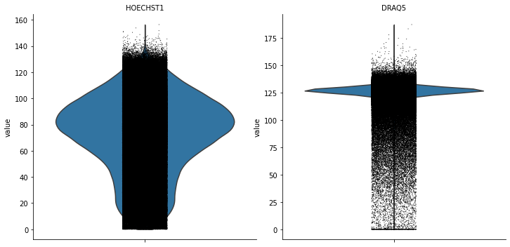
[8]:
# Remove cells with low DAPI intensity (most likely artifacts)
adata = adata[adata[:, "HOECHST1"].X > 60, :]
adata = adata[adata[:, "DRAQ5"].X > 100, :]
[9]:
# Remove the empty and nuclear channels
keep = [
    "CD44 - stroma",
    "FOXP3 - regulatory T cells",
    "CD8 - cytotoxic T cells",
    "p53 - tumor suppressor",
    "GATA3 - Th2 helper T cells",
    "CD45 - hematopoietic cells",
    "T-bet - Th1 cells",
    "beta-catenin - Wnt signaling",
    "HLA-DR - MHC-II",
    "PD-L1 - checkpoint",
    "Ki67 - proliferation",
    "CD45RA - naive T cells",
    "CD4 - T helper cells",
    "MUC-1 - epithelia",
    "CD30 - costimulator",
    "CD2 - T cells",
    "Vimentin - cytoplasm",
    "CD20 - B cells",
    "LAG-3 - checkpoint",
    "Na-K-ATPase - membranes",
    "CD5 - T cells",
    "IDO-1 - metabolism",
    "Cytokeratin - epithelia",
    "CD11b - macrophages",
    "CD56 - NK cells",
    "aSMA - smooth muscle",
    "BCL-2 - apoptosis",
    "CD25 - IL-2 Ra",
    "PD-1 - checkpoint",
    "Granzyme B - cytotoxicity",
    "EGFR - singling",
    "VISTA - costimulator",
    "CD15 - granulocytes",
    "ICOS - costimulator",
    "Synaptophysin - neuroendocrine",
    "GFAP - nerves",
    "CD7 - T cells",
    "CD3 - T cells",
    "Chromogranin A - neuroendocrine",
    "CD163 - macrophages",
    "CD45RO - memory cells",
    "CD68 - macrophages",
    "CD31 - vasculature",
    "Podoplanin - lymphatics",
    "CD34 - vasculature",
    "CD38 - multifunctional",
    "CD138 - plasma cells",
]
adata = adata[:, keep]
[10]:
adata_combined
[10]:
View of AnnData object with n_obs × n_vars = 272829 × 47
    obs: 'Region', 'coords', 'euler_number', 'filled_area', 'slice', 'tile', 'x', 'y', 'TMA'
    obsm: 'spatial'
    layers: 'max_intensity', 'min_intensity'
[11]:
# Rename the markers
adata.var_names = [
    "CD44",
    "FOXP3",
    "CD8",
    "p53",
    "GATA3",
    "CD45",
    "T-bet",
    "beta-cat",
    "HLA-DR",
    "PD-L1",
    "Ki67",
    "CD45RA",
    "CD4",
    "MUC-1",
    "CD30",
    "CD2",
    "Vimentin",
    "CD20",
    "LAG-3",
    "Na-K-ATPase",
    "CD5",
    "IDO-1",
    "Cytokeratin",
    "CD11b",
    "CD56",
    "aSMA",
    "BCL-2",
    "CD25-IL-2Ra",
    "PD-1",
    "Granzyme B",
    "EGFR",
    "VISTA",
    "CD15",
    "ICOS",
    "Synaptophysin",
    "GFAP",
    "CD7",
    "CD3",
    "ChromograninA",
    "CD163",
    "CD45RO",
    "CD68",
    "CD31",
    "Podoplanin",
    "CD34",
    "CD38",
    "CD138",
]
[12]:
# store the raw data for further use (differential expression or other analysis that uses raw counts)
adata.raw = adata
[13]:
## Add patients and groups info:
# Annotation dict for patients (the public data does not provide an easy way to map samples to phenotypes)
regions_to_patients = dict(
    reg001_A="1",
    reg001_B="1",
    reg002_A="1",
    reg002_B="1",
    reg003_A="2",
    reg003_B="2",
    reg004_A="2",
    reg004_B="2",
    reg005_A="3",
    reg005_B="3",
    reg006_A="3",
    reg006_B="3",
    reg007_A="4",
    reg007_B="4",
    reg008_A="4",
    reg008_B="4",
    reg009_A="5",
    reg009_B="5",
    reg010_A="5",
    reg010_B="5",
    reg011_A="6",
    reg011_B="6",
    reg012_A="6",
    reg012_B="6",
    reg013_A="7",
    reg013_B="7",
    reg014_A="7",
    reg014_B="7",
    reg015_A="8",
    reg015_B="8",
    reg016_A="8",
    reg016_B="8",
    reg017_A="9",
    reg017_B="9",
    reg018_A="9",
    reg018_B="9",
    reg019_A="10",
    reg019_B="10",
    reg020_A="10",
    reg020_B="10",
    reg021_A="11",
    reg021_B="11",
    reg022_A="11",
    reg022_B="11",
    reg023_A="12",
    reg023_B="12",
    reg024_A="12",
    reg024_B="12",
    reg025_A="13",
    reg025_B="13",
    reg026_A="13",
    reg026_B="13",
    reg027_A="14",
    reg027_B="14",
    reg028_A="14",
    reg028_B="14",
    reg029_A="15",
    reg029_B="15",
    reg030_A="15",
    reg030_B="15",
    reg031_A="16",
    reg031_B="16",
    reg032_A="16",
    reg032_B="16",
    reg033_A="17",
    reg033_B="17",
    reg034_A="17",
    reg034_B="17",
    reg035_A="18",
    reg035_B="18",
    reg036_A="18",
    reg036_B="18",
    reg037_A="19",
    reg037_B="19",
    reg038_A="19",
    reg038_B="19",
    reg039_A="20",
    reg039_B="20",
    reg040_A="20",
    reg040_B="20",
    reg041_A="21",
    reg041_B="21",
    reg042_A="21",
    reg042_B="21",
    reg043_A="22",
    reg043_B="22",
    reg044_A="22",
    reg044_B="22",
    reg045_A="23",
    reg045_B="23",
    reg046_A="23",
    reg046_B="23",
    reg047_A="24",
    reg047_B="24",
    reg048_A="24",
    reg048_B="24",
    reg049_A="25",
    reg049_B="25",
    reg050_A="25",
    reg050_B="25",
    reg051_A="26",
    reg051_B="26",
    reg052_A="26",
    reg052_B="26",
    reg053_A="27",
    reg053_B="27",
    reg054_A="27",
    reg054_B="27",
    reg055_A="28",
    reg055_B="28",
    reg056_A="28",
    reg056_B="28",
    reg057_A="29",
    reg057_B="29",
    reg058_A="29",
    reg058_B="29",
    reg059_A="30",
    reg059_B="30",
    reg060_A="30",
    reg060_B="30",
    reg061_A="31",
    reg061_B="31",
    reg062_A="31",
    reg062_B="31",
    reg063_A="32",
    reg063_B="32",
    reg064_A="32",
    reg064_B="32",
    reg065_A="33",
    reg065_B="33",
    reg066_A="33",
    reg066_B="33",
    reg067_A="34",
    reg067_B="34",
    reg068_A="34",
    reg068_B="34",
    reg069_A="35",
    reg069_B="35",
    reg070_A="35",
    reg070_B="35",
)
Annotation dict for clinical groups: - CLR: Crohns like reaction - DII: Diffuse inflammatory infiltrate
[14]:
regions_to_groups = dict(
    reg001_A="CLR",
    reg001_B="CLR",
    reg002_A="CLR",
    reg002_B="CLR",
    reg003_A="DII",
    reg003_B="DII",
    reg004_A="DII",
    reg004_B="DII",
    reg005_A="DII",
    reg005_B="DII",
    reg006_A="DII",
    reg006_B="DII",
    reg007_A="DII",
    reg007_B="DII",
    reg008_A="DII",
    reg008_B="DII",
    reg009_A="DII",
    reg009_B="DII",
    reg010_A="DII",
    reg010_B="DII",
    reg011_A="CLR",
    reg011_B="CLR",
    reg012_A="CLR",
    reg012_B="CLR",
    reg013_A="DII",
    reg013_B="DII",
    reg014_A="DII",
    reg014_B="DII",
    reg015_A="DII",
    reg015_B="DII",
    reg016_A="DII",
    reg016_B="DII",
    reg017_A="DII",
    reg017_B="DII",
    reg018_A="DII",
    reg018_B="DII",
    reg019_A="CLR",
    reg019_B="CLR",
    reg020_A="CLR",
    reg020_B="CLR",
    reg021_A="CLR",
    reg021_B="CLR",
    reg022_A="CLR",
    reg022_B="CLR",
    reg023_A="CLR",
    reg023_B="CLR",
    reg024_A="CLR",
    reg024_B="CLR",
    reg025_A="CLR",
    reg025_B="CLR",
    reg026_A="CLR",
    reg026_B="CLR",
    reg027_A="DII",
    reg027_B="DII",
    reg028_A="DII",
    reg028_B="DII",
    reg029_A="DII",
    reg029_B="DII",
    reg030_A="DII",
    reg030_B="DII",
    reg031_A="DII",
    reg031_B="DII",
    reg032_A="DII",
    reg032_B="DII",
    reg033_A="CLR",
    reg033_B="CLR",
    reg034_A="CLR",
    reg034_B="CLR",
    reg035_A="DII",
    reg035_B="DII",
    reg036_A="DII",
    reg036_B="DII",
    reg037_A="CLR",
    reg037_B="CLR",
    reg038_A="CLR",
    reg038_B="CLR",
    reg039_A="CLR",
    reg039_B="CLR",
    reg040_A="CLR",
    reg040_B="CLR",
    reg041_A="CLR",
    reg041_B="CLR",
    reg042_A="CLR",
    reg042_B="CLR",
    reg043_A="DII",
    reg043_B="DII",
    reg044_A="DII",
    reg044_B="DII",
    reg045_A="DII",
    reg045_B="DII",
    reg046_A="DII",
    reg046_B="DII",
    reg047_A="CLR",
    reg047_B="CLR",
    reg048_A="CLR",
    reg048_B="CLR",
    reg049_A="DII",
    reg049_B="DII",
    reg050_A="DII",
    reg050_B="DII",
    reg051_A="DII",
    reg051_B="DII",
    reg052_A="DII",
    reg052_B="DII",
    reg053_A="DII",
    reg053_B="DII",
    reg054_A="DII",
    reg054_B="DII",
    reg055_A="CLR",
    reg055_B="CLR",
    reg056_A="CLR",
    reg056_B="CLR",
    reg057_A="CLR",
    reg057_B="CLR",
    reg058_A="CLR",
    reg058_B="CLR",
    reg059_A="DII",
    reg059_B="DII",
    reg060_A="DII",
    reg060_B="DII",
    reg061_A="DII",
    reg061_B="DII",
    reg062_A="DII",
    reg062_B="DII",
    reg063_A="CLR",
    reg063_B="CLR",
    reg064_A="CLR",
    reg064_B="CLR",
    reg065_A="CLR",
    reg065_B="CLR",
    reg066_A="CLR",
    reg066_B="CLR",
    reg067_A="CLR",
    reg067_B="CLR",
    reg068_A="CLR",
    reg068_B="CLR",
    reg069_A="CLR",
    reg069_B="CLR",
    reg070_A="CLR",
    reg070_B="CLR",
)
[15]:
# map each slide to its source patient and clinical group (CLR vs DII)
adata.obs["patients"] = adata.obs["Region"].map(regions_to_patients).astype("category")

adata.obs["groups"] = adata.obs["Region"].map(regions_to_groups).astype("category")
[18]:
# log transform and scale the data
sc.pp.log1p(adata)
sc.pp.scale(adata, max_value=10)
[19]:
# PCA and batch correction using Harmony
sc.tl.pca(adata)
sc.external.pp.harmony_integrate(adata, key="Region")
2021-08-14 23:23:40,665 - harmonypy - INFO - Iteration 1 of 10
2021-08-14 23:26:19,392 - harmonypy - INFO - Iteration 2 of 10
2021-08-14 23:29:16,153 - harmonypy - INFO - Iteration 3 of 10
2021-08-14 23:32:22,647 - harmonypy - INFO - Converged after 3 iterations
[20]:
# save for future use
adata.write(filename="./data/adata_harmony.h5ad")
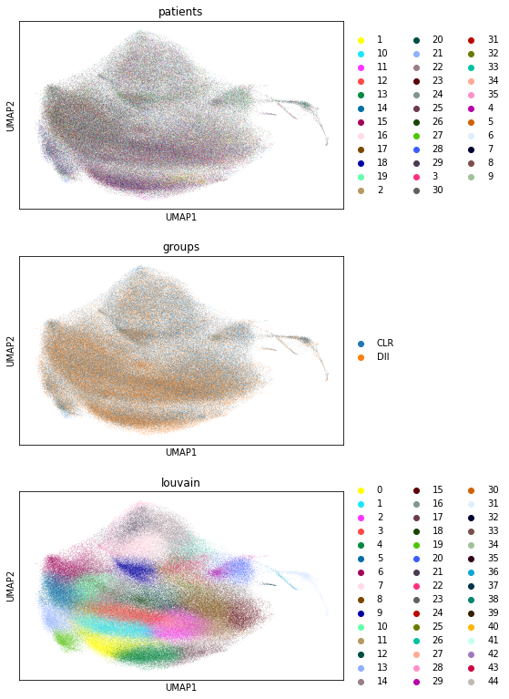
[21]:
# Compute neighbors and UMAP embedding
sc.pp.neighbors(adata, n_neighbors=15, n_pcs=30, use_rep="X_pca_harmony")
sc.tl.umap(adata)
[22]:
# louvain clustering
with parallel_backend("threading", n_jobs=15):
    sc.tl.louvain(adata, resolution=3)
[26]:
# Plot UMAP
sc.pl.umap(adata, color=["patients", "groups", "louvain"], ncols=1)
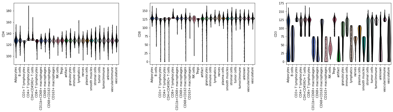
Annotate the clusters based on the markers intensity
Here, we define a function for cell annotation which takes as input the processed adata object together with a set of thresholds for each marker/channel. The function annotates the cells based on the specified thresholds and return the annotated adata object with the cell coordinates.
[27]:
def phenotype(adata, annot_dict):
    """
    Given a dict of dicts including phenotypes and marker gene thresholds, phenotype cells.

    Args:
        adata : the anndata object.
        annot_dict (dict): annotation dictionary each key is a cell type of interest and
            its value is a dictionary indicating protein expression ranges for that cell type.
            Each value should be a tuple (min, max) containing the minimum and maximum thresholds.
    """

    # Get the count matrix
    data = adata.copy()
    countMat = data.to_df()

    # Annotate the cell types
    for label in annot_dict.keys():
        for key, value in annot_dict[label].items():
            cond = np.logical_and.reduce(
                [
                    (
                        (countMat[k] >= countMat[k].quantile(list(v)[0]))
                        & (countMat[k] <= countMat[k].quantile(list(v)[1]))
                    )
                    for k, v in annot_dict[label].items()
                ]
            )
            data.obs.loc[cond, "cell_types"] = label
            # replace nan with unknown
            data.obs.cell_types.fillna("unknown", inplace=True)

    return data
[30]:
annot_dict = {
    "CD3+ T lymphocytes": {"CD3": (0.85, 1.0), "CD4": (0.0, 0.50), "CD8": (0.00, 0.50)},
    "CD4+ T lymphocytes": {
        "CD3": (0.50, 1.0),
        "CD4": (0.50, 1.0),
        "CD8": (0.0, 0.75),
        "CD45RO": (0.0, 0.75),
    },
    "CD8+ T lymphocytes": {"CD3": (0.50, 1), "CD8": (0.50, 1), "CD4": (0.0, 0.75)},
    "CD4+CD45RO+ T cells": {
        "CD3": (0.50, 1),
        "CD8": (0.0, 0.75),
        "CD4": (0.50, 1),
        "CD45RO": (0.50, 1),
    },
    "Tregs": {
        "CD3": (0.50, 1.0),
        "CD25-IL-2Ra": (0.75, 1),
        "FOXP3": (0.75, 1),
        "CD8": (0.0, 0.50),
    },
    "B cells": {"CD20": (0.50, 1), "CD3": (0.0, 0.75)},
    "plasma cells": {"CD38": (0.50, 1), "CD20": (0.50, 1), "CD3": (0.0, 0.75)},
    "granulocytes": {"CD15": (0.50, 1), "CD11b": (0.50, 1), "CD3": (0.0, 0.85)},
    "CD68+ macrophages": {"CD68": (0.95, 1), "CD3": (0.0, 0.50), "CD163": (0.0, 0.95)},
    "CD163+ macrophages": {"CD163": (0.95, 1), "CD3": (0.0, 0.50), "CD68": (0.0, 0.50)},
    "CD68+CD163 macrophages": {
        "CD68": (0.50, 1),
        "CD163": (0.50, 1),
        "CD3": (0.0, 0.95),
    },
    "CD11b+CD68+ macrophages": {
        "CD68": (0.95, 1),
        "CD11b": (0.50, 1),
        "CD3": (0.0, 0.50),
    },
    "NK cells": {"CD56": (0.75, 1), "CD3": (0.0, 0.50), "Cytokeratin": (0.0, 0.50)},
    "vasculature": {"CD34": (0.50, 1), "CD31": (0.50, 1), "Cytokeratin": (0.0, 0.50)},
    "tumor cells": {"Cytokeratin": (0.50, 1), "p53": (0.50, 1), "aSMA": (0.0, 0.75)},
    "immune cells": {
        "CD20": (0.50, 1),
        "CD38": (0.50, 1),
        "CD3": (0.50, 1),
        "GFAP": (0.50, 1),
        "CD15": (0.50, 1),
        "Cytokeratin": (0.0, 0.50),
        "aSMA": (0.0, 0.75),
    },
    "tumor/immune": {
        "CD20": (0.50, 1),
        "CD3": (0.75, 1),
        "CD38": (0.50, 1),
        "GFAP": (0.80, 1),
        "Cytokeratin": (0.85, 1),
        "p53": (0.50, 1),
        "aSMA": (0.0, 0.75),
    },
    "vascular/immune": {
        "CD20": (0.50, 1),
        "CD3": (0.85, 1),
        "CD38": (0.50, 1),
        "GFAP": (0.80, 1),
        "CD34": (0.75, 1),
        "CD31": (0.75, 1),
        "aSMA": (0.0, 0.75),
    },
    "stromal cells": {"Vimentin": (0.50, 1), "Cytokeratin": (0.0, 0.50)},
    "Adipocytes": {
        "p53": (0.75, 1),
        "Vimentin": (0.75, 1),
        "Cytokeratin": (0.0, 0.50),
        "aSMA": (0.0, 0.50),
        "CD44": (0.0, 0.50),
    },
    "smooth muscles": {"aSMA": (0.70, 1), "Vimentin": (0.50, 1), "CD3": (0.0, 0.50)},
    "nerves": {
        "Synaptophysin": (0.85, 1),
        "Vimentin": (0.50, 1),
        "GFAP": (0.85, 1),
        "CD3": (0.0, 0.50),
    },
    "lymphatics": {"Podoplanin": (0.99, 1), "CD3": (0.0, 0.75)},
    "artifact": {
        "CD20": (0.0, 0.50),
        "CD3": (0.0, 0.50),
        "CD38": (0.0, 0.50),
        "GFAP": (0.0, 0.50),
        "Cytokeratin": (0.0, 0.50),
        "p53": (0.0, 0.50),
        "aSMA": (0.0, 0.50),
        "CD15": (0.0, 0.50),
        "CD68": (0.0, 0.50),
        "CD25-IL-2Ra": (0.0, 0.50),
        "CD34": (0.0, 0.50),
        "CD31": (0.0, 0.50),
        "CD56": (0.0, 0.50),
        "Vimentin": (0.0, 0.50),
    },
}
[31]:
# Annotate the adata
adata_annot = process_adata(adata, annot_dict=annot_dict)
adata_annot.obs.cell_types.value_counts()
[31]:
unknown                    42834
tumor cells                37035
stromal cells              31646
CD68+CD163 macrophages     28479
granulocytes               23164
vasculature                20016
smooth muscles             19990
B cells                    13433
CD8+ T lymphocytes         10962
plasma cells                8911
CD4+CD45RO+ T cells         6603
artifact                    4650
CD4+ T lymphocytes          4395
vascular/immune             4004
CD3+ T lymphocytes          3975
immune cells                3075
Adipocytes                  2825
tumor/immune                1925
CD68+ macrophages           1431
Tregs                       1067
CD11b+CD68+ macrophages      869
lymphatics                   865
nerves                       366
CD163+ macrophages           220
NK cells                      89
Name: cell_types, dtype: int64
[33]:
sc.pl.violin(adata_annot, groupby="cell_types", keys=["CD4", "CD8", "CD3"], rotation=90)
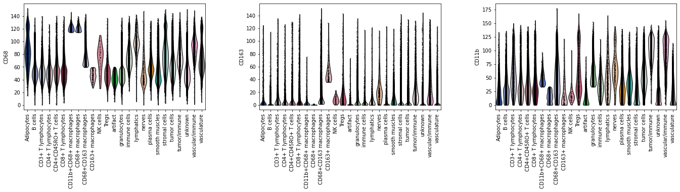
[35]:
sc.pl.violin(
    adata_annot, groupby="cell_types", keys=["CD68", "CD163", "CD11b"], rotation=90
)
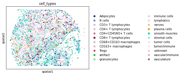
[36]:
sc.pl.spatial(
    adata_annot[adata_annot.obs.Region == "reg020_A"],
    color="cell_types",
    spot_size=25,
    size=1,
)
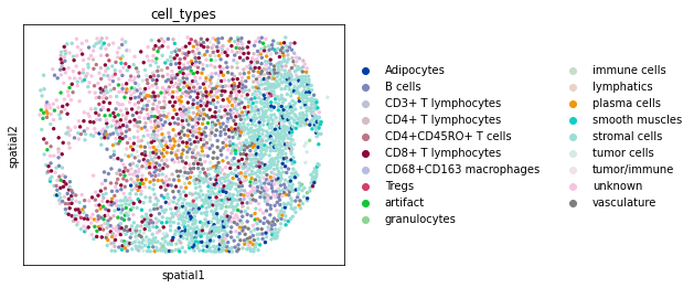
[37]:
sc.pl.spatial(
    adata_annot[adata_annot.obs.Region == "reg020_B"],
    color="cell_types",
    spot_size=25,
    size=1,
)
[39]:
# Put in a dataframe for further analysis
countData = adata_annot.to_df()
obs = adata_annot.obs
data = pd.concat([countData, obs], axis = 1)
data['CellID'] = Data.index\# Remove the cells with unknown annotation and the artifacts
data = data.loc[~Data['cell_types'].isin(['unknown'])]
data = data.loc[~Data['cell_types'].isin(['artifact'])]
data['cell_types'] = data['cell_types'].cat.remove_unused_categories()
data['cell_types'] = data['cell_types'].astype('str')
[44]:
data.shape
[44]:
(225345, 61)
[45]:
# save
data.to_csv("./data/CRC_pathml.csv")
Identification of cellular neighborhoods
After identifying cell types, the next step is to identify cellular neighborhoods using the same approach described in Schürch et. al. and utilizing the code available from: https://github.com/nolanlab/NeighborhoodCoordination
In summary, for each cell, we are going to idenify the 10 nearest spatial neighbors (windows), then we are going to cluster these windows into distinct neighborhoods based on their cell type composition.
[46]:
from sklearn.neighbors import NearestNeighbors
import time
import sys
from sklearn.cluster import MiniBatchKMeans
import seaborn as sns
[47]:
# Function for identifying the windows
def get_windows(job, n_neighbors):
    """
    For each region and each individual cell in dataset, return the indices of the nearest neighbors.

    'job:  meta data containing the start time,index of region, region name, indices of region in original dataframe
    n_neighbors:  the number of neighbors to find for each cell
    """
    start_time, idx, tissue_name, indices = job
    job_start = time.time()

    print("Starting:", str(idx + 1) + "/" + str(len(exps)), ": " + exps[idx])

    # tissue_group: a grouped data frame with X and Y coordinates grouped by unique tissue regions
    tissue = tissue_group.get_group(tissue_name)

    to_fit = tissue.loc[indices][["x", "y"]].values

    # Unsupervised learner for implementing neighbor searches.
    fit = NearestNeighbors(n_neighbors=n_neighbors).fit(tissue[["x", "y"]].values)

    # Find the nearest neighbors

    m = fit.kneighbors(to_fit)

    m = m[0], m[1]

    ## sort_neighbors
    args = m[0].argsort(axis=1)

    add = np.arange(m[1].shape[0]) * m[1].shape[1]

    sorted_indices = m[1].flatten()[args + add[:, None]]

    neighbors = tissue.index.values[sorted_indices]

    end_time = time.time()

    print(
        "Finishing:",
        str(idx + 1) + "/" + str(len(exps)),
        ": " + exps[idx],
        end_time - job_start,
        end_time - start_time,
    )
    return neighbors.astype(np.int32)
[48]:
data = pd.read_csv("./data/CRC_pathml.csv")
[49]:
# make dummy variables
data = pd.concat([Data, pd.get_dummies(Data["cell_types"])], axis=1)
# Extract the cell types with dummy variables
sum_cols = data["cell_types"].unique()
values = data[sum_cols].values
find windows for each cell in each tissue region
[51]:
# Keep the X and Y coordianates + the tissue regions >> then group by tissue regions (140 unique regions)
tissue_group = data[["x", "y", "Region"]].groupby("Region")

# Create a list of unique tissue regions
exps = list(data["Region"].unique())

# time.time(): current time is seconds
# indices: a list of indices (rownames) of each dataframe in tissue_group
# exps.index(t) : t represents the index of each one of the indices eg, exps.index("reg001_A") is 0 and exps.index("reg001_B") is 1 and so on
# t is the name of tissue regions eg, reg001_A
tissue_chunks = [
    (time.time(), exps.index(t), t, a)
    for t, indices in tissue_group.groups.items()
    for a in np.array_split(indices, 1)
]

# Get the window (the 10 closest cells to each cell in each tissue region)
tissues = [get_windows(job, 10) for job in tissue_chunks]
Starting: 61/140 : reg001_A
Finishing: 61/140 : reg001_A 0.009814977645874023 0.022227048873901367
Starting: 77/140 : reg001_B
Finishing: 77/140 : reg001_B 0.004416942596435547 0.026772260665893555
Starting: 19/140 : reg002_A
Finishing: 19/140 : reg002_A 0.006669044494628906 0.0336461067199707
Starting: 101/140 : reg002_B
Finishing: 101/140 : reg002_B 0.0061969757080078125 0.04012012481689453
Starting: 58/140 : reg003_A
Finishing: 58/140 : reg003_A 0.005404233932495117 0.045838117599487305
Starting: 85/140 : reg003_B
Finishing: 85/140 : reg003_B 0.002471923828125 0.04852771759033203
Starting: 65/140 : reg004_A
Finishing: 65/140 : reg004_A 0.005899906158447266 0.054521799087524414
Starting: 71/140 : reg004_B
Finishing: 71/140 : reg004_B 0.0063402652740478516 0.06109809875488281
Starting: 40/140 : reg005_A
Finishing: 40/140 : reg005_A 0.0077631473541259766 0.0690910816192627
Starting: 105/140 : reg005_B
Finishing: 105/140 : reg005_B 0.005625247955322266 0.07496023178100586
Starting: 8/140 : reg006_A
Finishing: 8/140 : reg006_A 0.004698991775512695 0.0797572135925293
Starting: 127/140 : reg006_B
Finishing: 127/140 : reg006_B 0.004808902740478516 0.08475184440612793
Starting: 17/140 : reg007_A
Finishing: 17/140 : reg007_A 0.007723093032836914 0.09262681007385254
Starting: 92/140 : reg007_B
Finishing: 92/140 : reg007_B 0.0049021244049072266 0.09776902198791504
Starting: 24/140 : reg008_A
Finishing: 24/140 : reg008_A 0.005953073501586914 0.1038961410522461
Starting: 123/140 : reg008_B
Finishing: 123/140 : reg008_B 0.008786916732788086 0.11287188529968262
Starting: 52/140 : reg009_A
Finishing: 52/140 : reg009_A 0.0069849491119384766 0.12202978134155273
Starting: 130/140 : reg009_B
Finishing: 130/140 : reg009_B 0.0077838897705078125 0.12995290756225586
Starting: 12/140 : reg010_A
Finishing: 12/140 : reg010_A 0.006242036819458008 0.13639497756958008
Starting: 133/140 : reg010_B
Finishing: 133/140 : reg010_B 0.003675222396850586 0.14031219482421875
Starting: 23/140 : reg011_A
Finishing: 23/140 : reg011_A 0.004063129425048828 0.1445319652557373
Starting: 124/140 : reg011_B
Finishing: 124/140 : reg011_B 0.00393986701965332 0.14860916137695312
Starting: 69/140 : reg012_A
Finishing: 69/140 : reg012_A 0.005756855010986328 0.15452790260314941
Starting: 75/140 : reg012_B
Finishing: 75/140 : reg012_B 0.0026569366455078125 0.15730595588684082
Starting: 41/140 : reg013_A
Finishing: 41/140 : reg013_A 0.0051670074462890625 0.16249799728393555
Starting: 108/140 : reg013_B
Finishing: 108/140 : reg013_B 0.00403904914855957 0.1666700839996338
Starting: 44/140 : reg014_A
Finishing: 44/140 : reg014_A 0.003408193588256836 0.17021417617797852
Starting: 98/140 : reg014_B
Finishing: 98/140 : reg014_B 0.005333900451660156 0.1755669116973877
Starting: 54/140 : reg015_A
Finishing: 54/140 : reg015_A 0.006878852844238281 0.18254685401916504
Starting: 88/140 : reg015_B
Finishing: 88/140 : reg015_B 0.004870891571044922 0.1875441074371338
Starting: 29/140 : reg016_A
Finishing: 29/140 : reg016_A 0.006279945373535156 0.19389891624450684
Starting: 107/140 : reg016_B
Finishing: 107/140 : reg016_B 0.00708317756652832 0.20116114616394043
Starting: 67/140 : reg017_A
Finishing: 67/140 : reg017_A 0.006649971008300781 0.20815491676330566
Starting: 72/140 : reg017_B
Finishing: 72/140 : reg017_B 0.005545854568481445 0.21404600143432617
Starting: 4/140 : reg018_A
Finishing: 4/140 : reg018_A 0.008655071258544922 0.2230057716369629
Starting: 78/140 : reg018_B
Finishing: 78/140 : reg018_B 0.006451129913330078 0.2296450138092041
Starting: 32/140 : reg019_A
Finishing: 32/140 : reg019_A 0.006360054016113281 0.23619771003723145
Starting: 113/140 : reg019_B
Finishing: 113/140 : reg019_B 0.003787994384765625 0.24015522003173828
Starting: 60/140 : reg020_A
Finishing: 60/140 : reg020_A 0.010369062423706055 0.2506411075592041
Starting: 138/140 : reg020_B
Finishing: 138/140 : reg020_B 0.008259773254394531 0.25922179222106934
Starting: 39/140 : reg021_A
Finishing: 39/140 : reg021_A 0.004830837249755859 0.2642190456390381
Starting: 116/140 : reg021_B
Finishing: 116/140 : reg021_B 0.003367900848388672 0.26804184913635254
Starting: 9/140 : reg022_A
Finishing: 9/140 : reg022_A 0.007760047912597656 0.27587199211120605
Starting: 126/140 : reg022_B
Finishing: 126/140 : reg022_B 0.0032799243927001953 0.27936792373657227
Starting: 20/140 : reg023_A
Finishing: 20/140 : reg023_A 0.004238128662109375 0.283825159072876
Starting: 93/140 : reg023_B
Finishing: 93/140 : reg023_B 0.005738973617553711 0.2899298667907715
Starting: 33/140 : reg024_A
Finishing: 33/140 : reg024_A 0.002911806106567383 0.2929408550262451
Starting: 112/140 : reg024_B
Finishing: 112/140 : reg024_B 0.013455867767333984 0.30647897720336914
Starting: 62/140 : reg025_A
Finishing: 62/140 : reg025_A 0.006231069564819336 0.313082218170166
Starting: 76/140 : reg025_B
Finishing: 76/140 : reg025_B 0.009344816207885742 0.3225746154785156
Starting: 50/140 : reg026_A
Finishing: 50/140 : reg026_A 0.0073397159576416016 0.3299558162689209
Starting: 95/140 : reg026_B
Finishing: 95/140 : reg026_B 0.010460853576660156 0.34046483039855957
Starting: 57/140 : reg027_A
Finishing: 57/140 : reg027_A 0.008396148681640625 0.3488960266113281
Starting: 81/140 : reg027_B
Finishing: 81/140 : reg027_B 0.008210897445678711 0.3574059009552002
Starting: 14/140 : reg028_A
Finishing: 14/140 : reg028_A 0.007547855377197266 0.3653140068054199
Starting: 87/140 : reg028_B
Finishing: 87/140 : reg028_B 0.00654292106628418 0.3718750476837158
Starting: 46/140 : reg029_A
Finishing: 46/140 : reg029_A 0.009541988372802734 0.38150620460510254
Starting: 104/140 : reg029_B
Finishing: 104/140 : reg029_B 0.006811857223510742 0.38849782943725586
Starting: 47/140 : reg030_A
Finishing: 47/140 : reg030_A 0.003790140151977539 0.39242005348205566
Starting: 99/140 : reg030_B
Finishing: 99/140 : reg030_B 0.006364107131958008 0.39893221855163574
Starting: 53/140 : reg031_A
Finishing: 53/140 : reg031_A 0.004971981048583984 0.4040391445159912
Starting: 128/140 : reg031_B
Finishing: 128/140 : reg031_B 0.006245851516723633 0.41039395332336426
Starting: 28/140 : reg032_A
Finishing: 28/140 : reg032_A 0.006634950637817383 0.4171791076660156
Starting: 106/140 : reg032_B
Finishing: 106/140 : reg032_B 0.004702329635620117 0.4219231605529785
Starting: 1/140 : reg033_A
Finishing: 1/140 : reg033_A 0.008253097534179688 0.4303441047668457
Starting: 73/140 : reg033_B
Finishing: 73/140 : reg033_B 0.006574869155883789 0.43709278106689453
Starting: 15/140 : reg034_A
Finishing: 15/140 : reg034_A 0.006840944290161133 0.4440948963165283
Starting: 89/140 : reg034_B
Finishing: 89/140 : reg034_B 0.009439229965209961 0.45371532440185547
Starting: 25/140 : reg035_A
Finishing: 25/140 : reg035_A 0.008854866027832031 0.4627108573913574
Starting: 120/140 : reg035_B
Finishing: 120/140 : reg035_B 0.009293794631958008 0.47219085693359375
Starting: 68/140 : reg036_A
Finishing: 68/140 : reg036_A 0.009788990020751953 0.48207616806030273
Starting: 139/140 : reg036_B
Finishing: 139/140 : reg036_B 0.01093912124633789 0.49315786361694336
Starting: 43/140 : reg037_A
Finishing: 43/140 : reg037_A 0.005067110061645508 0.4984712600708008
Starting: 117/140 : reg037_B
Finishing: 117/140 : reg037_B 0.006145000457763672 0.5049071311950684
Starting: 38/140 : reg038_A
Finishing: 38/140 : reg038_A 0.006515026092529297 0.5115442276000977
Starting: 110/140 : reg038_B
Finishing: 110/140 : reg038_B 0.006800174713134766 0.5184721946716309
Starting: 59/140 : reg039_A
Finishing: 59/140 : reg039_A 0.003709077835083008 0.5222232341766357
Starting: 74/140 : reg039_B
Finishing: 74/140 : reg039_B 0.0035741329193115234 0.5277011394500732
Starting: 18/140 : reg040_A
Finishing: 18/140 : reg040_A 0.004296064376831055 0.5321159362792969
Starting: 96/140 : reg040_B
Finishing: 96/140 : reg040_B 0.004117727279663086 0.536341667175293
Starting: 7/140 : reg041_A
Finishing: 7/140 : reg041_A 0.003995180130004883 0.540438175201416
Starting: 82/140 : reg041_B
Finishing: 82/140 : reg041_B 0.003885030746459961 0.5444629192352295
Starting: 37/140 : reg042_A
Finishing: 37/140 : reg042_A 0.003648042678833008 0.548213005065918
Starting: 109/140 : reg042_B
Finishing: 109/140 : reg042_B 0.003875255584716797 0.552192211151123
Starting: 63/140 : reg043_A
Finishing: 63/140 : reg043_A 0.0053560733795166016 0.5576450824737549
Starting: 79/140 : reg043_B
Finishing: 79/140 : reg043_B 0.0034198760986328125 0.5609321594238281
Starting: 10/140 : reg044_A
Finishing: 10/140 : reg044_A 0.003528118133544922 0.5645391941070557
Starting: 131/140 : reg044_B
Finishing: 131/140 : reg044_B 0.002878904342651367 0.5675170421600342
Starting: 21/140 : reg045_A
Finishing: 21/140 : reg045_A 0.01139378547668457 0.5790097713470459
Starting: 97/140 : reg045_B
Finishing: 97/140 : reg045_B 0.004516124725341797 0.58365797996521
Starting: 6/140 : reg046_A
Finishing: 6/140 : reg046_A 0.003998756408691406 0.5878088474273682
Starting: 134/140 : reg046_B
Finishing: 134/140 : reg046_B 0.01061391830444336 0.5984470844268799
Starting: 34/140 : reg047_A
Finishing: 34/140 : reg047_A 0.005155086517333984 0.6037991046905518
Starting: 118/140 : reg047_B
Finishing: 118/140 : reg047_B 0.007688999176025391 0.6116068363189697
Starting: 30/140 : reg048_A
Finishing: 30/140 : reg048_A 0.007600307464599609 0.6195840835571289
Starting: 115/140 : reg048_B
Finishing: 115/140 : reg048_B 0.011443138122558594 0.6316161155700684
Starting: 2/140 : reg049_A
Finishing: 2/140 : reg049_A 0.00881505012512207 0.6405959129333496
Starting: 135/140 : reg049_B
Finishing: 135/140 : reg049_B 0.011723041534423828 0.6528370380401611
Starting: 3/140 : reg050_A
Finishing: 3/140 : reg050_A 0.0052111148834228516 0.6582260131835938
Starting: 136/140 : reg050_B
Finishing: 136/140 : reg050_B 0.009176015853881836 0.6675820350646973
Starting: 31/140 : reg051_A
Finishing: 31/140 : reg051_A 0.008751153945922852 0.6764531135559082
Starting: 114/140 : reg051_B
Finishing: 114/140 : reg051_B 0.008320093154907227 0.68532395362854
Starting: 51/140 : reg052_A
Finishing: 51/140 : reg052_A 0.0061681270599365234 0.6917729377746582
Starting: 84/140 : reg052_B
Finishing: 84/140 : reg052_B 0.009895801544189453 0.7022178173065186
Starting: 45/140 : reg053_A
Finishing: 45/140 : reg053_A 0.004172086715698242 0.7066078186035156
Starting: 94/140 : reg053_B
Finishing: 94/140 : reg053_B 0.004163980484008789 0.7108440399169922
Starting: 27/140 : reg054_A
Finishing: 27/140 : reg054_A 0.005264997482299805 0.7162370681762695
Starting: 111/140 : reg054_B
Finishing: 111/140 : reg054_B 0.003180980682373047 0.7195639610290527
Starting: 66/140 : reg055_A
Finishing: 66/140 : reg055_A 0.00409388542175293 0.7237598896026611
Starting: 80/140 : reg055_B
Finishing: 80/140 : reg055_B 0.0030677318572998047 0.7269597053527832
Starting: 22/140 : reg056_A
Finishing: 22/140 : reg056_A 0.005424976348876953 0.7325129508972168
Starting: 125/140 : reg056_B
Finishing: 125/140 : reg056_B 0.011126041412353516 0.7440230846405029
Starting: 13/140 : reg057_A
Finishing: 13/140 : reg057_A 0.00240325927734375 0.7465171813964844
Starting: 132/140 : reg057_B
Finishing: 132/140 : reg057_B 0.004606008529663086 0.7512319087982178
Starting: 56/140 : reg058_A
Finishing: 56/140 : reg058_A 0.00801992416381836 0.7594480514526367
Starting: 129/140 : reg058_B
Finishing: 129/140 : reg058_B 0.007853984832763672 0.7673490047454834
Starting: 49/140 : reg059_A
Finishing: 49/140 : reg059_A 0.007686138153076172 0.775170087814331
Starting: 119/140 : reg059_B
Finishing: 119/140 : reg059_B 0.008450984954833984 0.7838461399078369
Starting: 11/140 : reg060_A
Finishing: 11/140 : reg060_A 0.007905006408691406 0.7919058799743652
Starting: 86/140 : reg060_B
Finishing: 86/140 : reg060_B 0.00969386100769043 0.8019630908966064
Starting: 16/140 : reg061_A
Finishing: 16/140 : reg061_A 0.007141828536987305 0.8094010353088379
Starting: 100/140 : reg061_B
Finishing: 100/140 : reg061_B 0.008517742156982422 0.8181126117706299
Starting: 64/140 : reg062_A
Finishing: 64/140 : reg062_A 0.008826017379760742 0.8272860050201416
Starting: 140/140 : reg062_B
Finishing: 140/140 : reg062_B 0.007968902587890625 0.83530592918396
Starting: 35/140 : reg063_A
Finishing: 35/140 : reg063_A 0.003358125686645508 0.8388819694519043
Starting: 122/140 : reg063_B
Finishing: 122/140 : reg063_B 0.005372285842895508 0.8444433212280273
Starting: 48/140 : reg064_A
Finishing: 48/140 : reg064_A 0.0074350833892822266 0.8521482944488525
Starting: 121/140 : reg064_B
Finishing: 121/140 : reg064_B 0.008898019790649414 0.8611080646514893
Starting: 55/140 : reg065_A
Finishing: 55/140 : reg065_A 0.00514674186706543 0.8664467334747314
Starting: 137/140 : reg065_B
Finishing: 137/140 : reg065_B 0.006044864654541016 0.8725459575653076
Starting: 26/140 : reg066_A
Finishing: 26/140 : reg066_A 0.003931999206542969 0.8765108585357666
Starting: 91/140 : reg066_B
Finishing: 91/140 : reg066_B 0.012857198715209961 0.889430046081543
Starting: 5/140 : reg067_A
Finishing: 5/140 : reg067_A 0.004929780960083008 0.8947200775146484
Starting: 83/140 : reg067_B
Finishing: 83/140 : reg067_B 0.004603862762451172 0.899526834487915
Starting: 70/140 : reg068_A
Finishing: 70/140 : reg068_A 0.003593921661376953 0.9033100605010986
Starting: 90/140 : reg068_B
Finishing: 90/140 : reg068_B 0.008028984069824219 0.9117860794067383
Starting: 42/140 : reg069_A
Finishing: 42/140 : reg069_A 0.004137992858886719 0.9161639213562012
Starting: 102/140 : reg069_B
Finishing: 102/140 : reg069_B 0.005839109420776367 0.9220380783081055
Starting: 36/140 : reg070_A
Finishing: 36/140 : reg070_A 0.0063631534576416016 0.92854905128479
Starting: 103/140 : reg070_B
Finishing: 103/140 : reg070_B 0.004929065704345703 0.9335160255432129
for each cell and its nearest neighbors, reshape and count the number of each cell type in those neighbors.
[52]:
ks = [10]
out_dict = {}
for k in ks:
    for neighbors, job in zip(tissues, tissue_chunks):
        chunk = np.arange(len(neighbors))  # indices
        tissue_name = job[2]
        indices = job[3]
        window = (
            values[neighbors[chunk, :k].flatten()]
            .reshape(len(chunk), k, len(sum_cols))
            .sum(axis=1)
        )
        out_dict[(tissue_name, k)] = (window.astype(np.float16), indices)
concatenate the summed windows and combine into one dataframe for each window size tested.
[53]:
keep_cols = ["x", "y", "Region", "cell_types"]
windows = {}
for k in ks:
    window = pd.concat(
        [
            pd.DataFrame(
                out_dict[(exp, k)][0],
                index=out_dict[(exp, k)][1].astype(int),
                columns=sum_cols,
            )
            for exp in exps
        ],
        0,
    )
    window = window.loc[Data.index.values]
    window = pd.concat([Data[keep_cols], window], 1)
    windows[k] = window
<ipython-input-53-dbc25edfe709>:4: FutureWarning: In a future version of pandas all arguments of concat except for the argument 'objs' will be keyword-only
  window = pd.concat(
<ipython-input-53-dbc25edfe709>:8: FutureWarning: In a future version of pandas all arguments of concat except for the argument 'objs' will be keyword-only
  window = pd.concat([Data[keep_cols], window], 1)
[54]:
neighborhood_name = "neighborhood" + str(k)
k_centroids = {}

windows2 = windows[10]
Clustering the windows
[64]:
km = MiniBatchKMeans(n_clusters=10, random_state=0)

labelskm = km.fit_predict(windows2[sum_cols].values)
k_centroids[10] = km.cluster_centers_
data["neighborhood10"] = labelskm
data[neighborhood_name] = data[neighborhood_name].astype("category")
[65]:
cell_order = [
    "tumor cells",
    "CD68+CD163 macrophages",
    "CD11b+CD68+ macrophages",
    "CD68+ macrophages",
    "CD163+ macrophages",
    "granulocytes",
    "NK cells",
    "CD3+ T lymphocytes",
    "CD4+ T lymphocytes",
    "CD4+CD45RO+ T cells",
    "CD8+ T lymphocytes",
    "Tregs",
    "B cells",
    "plasma cells",
    "tumor/immune",
    "vascular/immune",
    "immune cells",
    "smooth muscles",
    "stromal cells",
    "vasculature",
    "lymphatics",
    "nerves",
]
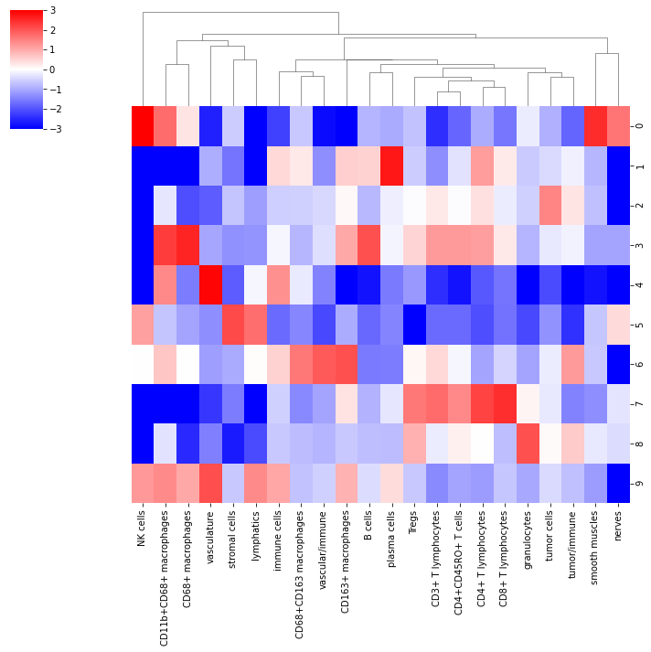
This plot shows the cell types abundance in the different niches
[66]:
niche_clusters = k_centroids[10]
tissue_avgs = values.mean(axis=0)
fc = np.log2(
    (
        (niche_clusters + tissue_avgs)
        / (niche_clusters + tissue_avgs).sum(axis=1, keepdims=True)
    )
    / tissue_avgs
)
fc = pd.DataFrame(fc, columns=sum_cols)
s = sns.clustermap(
    fc.loc[[0, 1, 2, 3, 4, 5, 6, 7, 8, 9], cell_order],
    vmin=-3,
    vmax=3,
    cmap="bwr",
    row_cluster=False,
)
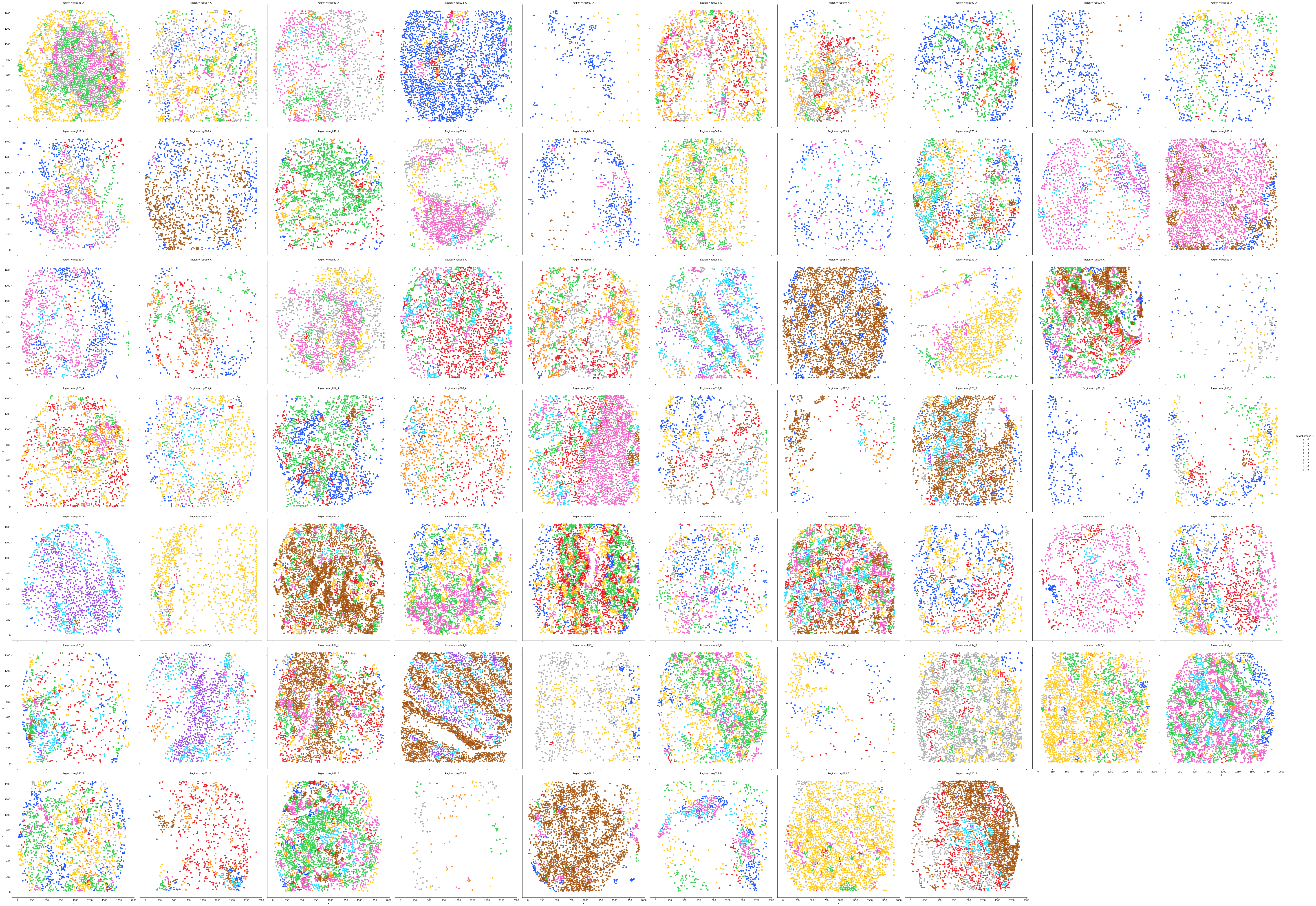
Visualize the identified neighborhoods on the slides in each clinical group
[67]:
# CLR
Data["neighborhood10"] = Data["neighborhood10"].astype("category")
sns.lmplot(
    data=Data[Data["groups"] == "CLR"],
    x="x",
    y="y",
    hue="neighborhood10",
    palette="bright",
    height=8,
    col="Region",
    col_wrap=10,
    fit_reg=False,
)
[67]:
<seaborn.axisgrid.FacetGrid at 0x1a79e42e0>
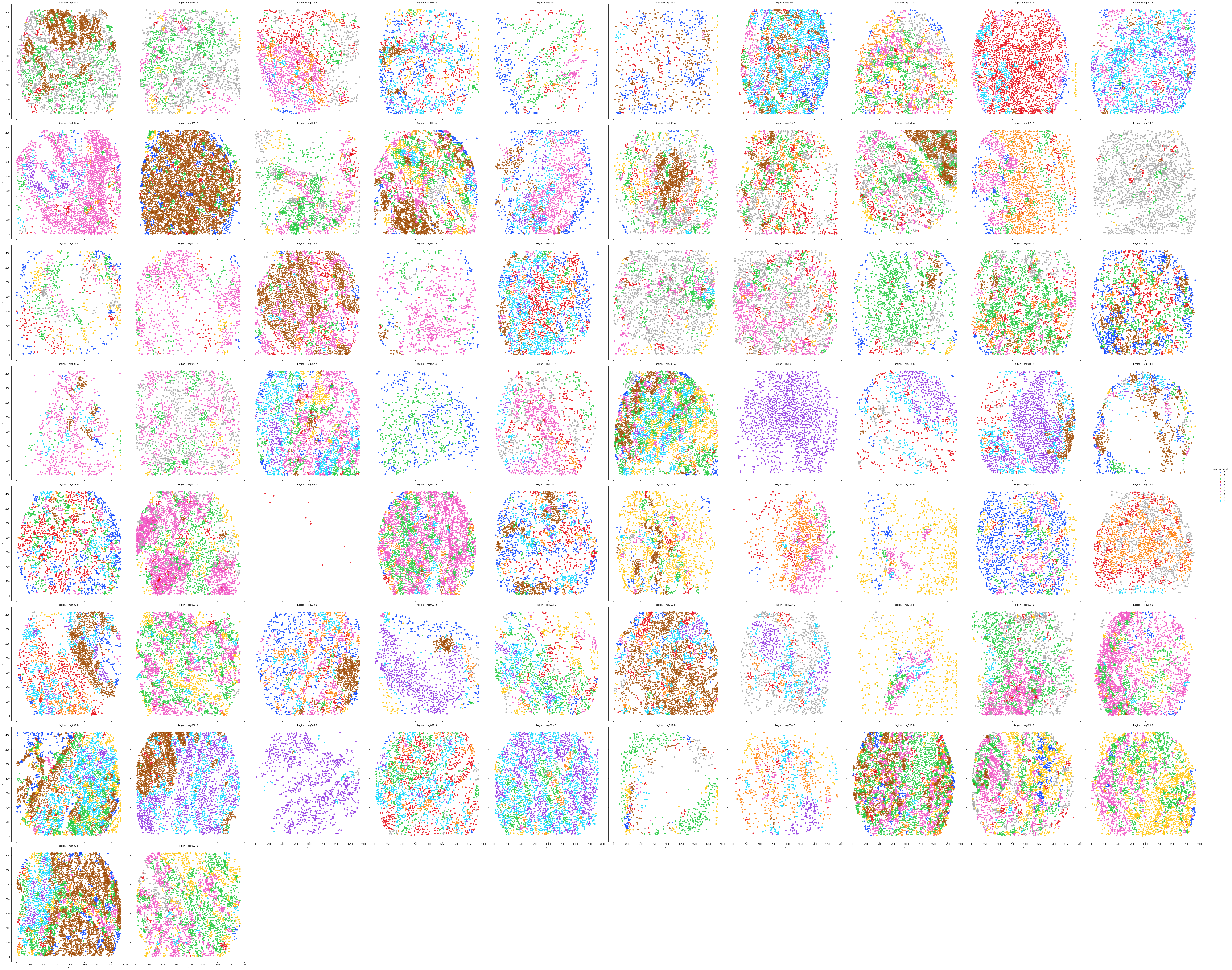
[68]:
# DII
Data["neighborhood10"] = Data["neighborhood10"].astype("category")
sns.lmplot(
    data=Data[Data["groups"] == "DII"],
    x="x",
    y="y",
    hue="neighborhood10",
    palette="bright",
    height=8,
    col="Region",
    col_wrap=10,
    fit_reg=False,
)
[68]:
<seaborn.axisgrid.FacetGrid at 0x1a78afc40>
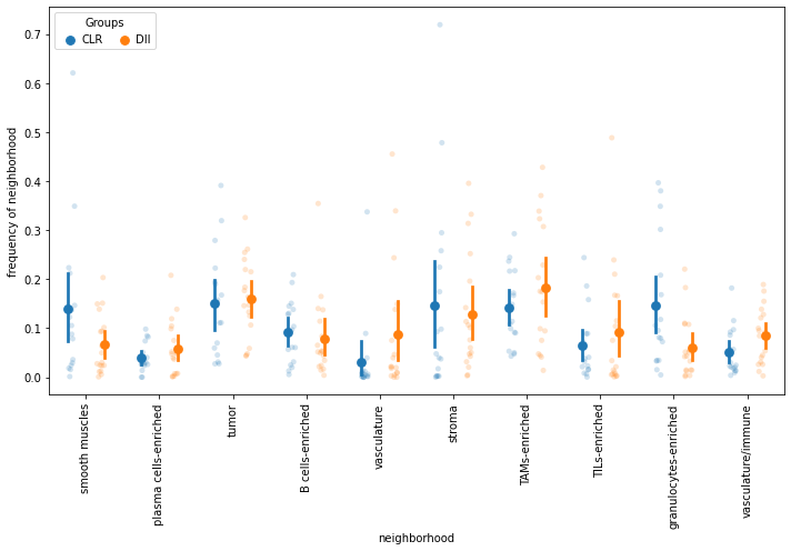
Plot for each group and each patient the percent of total cells allocated to each neighborhood
[70]:
fc = Data.groupby(["patients", "groups"]).apply(
    lambda x: x["neighborhood10"].value_counts(sort=False, normalize=True)
)

fc.columns = range(10)
melt = pd.melt(fc.reset_index(), id_vars=["patients", "groups"])
melt = melt.rename(
    columns={"variable": "neighborhood", "value": "frequency of neighborhood"}
)
melt["neighborhood"] = melt["neighborhood"].map(
    {
        0: "smooth muscles",
        1: "plasma cells-enriched",
        2: "tumor",
        3: "B cells-enriched",
        4: "vasculature",
        5: "stroma",
        6: "TAMs-enriched",
        7: "TILs-enriched",
        8: "granulocytes-enriched",
        9: "vasculature/immune",
    }
)

f, ax = plt.subplots(figsize=(10, 7))
sns.stripplot(
    data=melt,
    hue="groups",
    dodge=True,
    alpha=0.2,
    x="neighborhood",
    y="frequency of neighborhood",
)
sns.pointplot(
    data=melt,
    scatter_kws={"marker": "d"},
    hue="groups",
    dodge=0.5,
    join=False,
    x="neighborhood",
    y="frequency of neighborhood",
)
handles, labels = ax.get_legend_handles_labels()
plt.xticks(rotation=90, fontsize="10", ha="center")
ax.legend(
    handles[:2],
    labels[:2],
    title="Groups",
    handletextpad=0,
    columnspacing=1,
    loc="upper left",
    ncol=3,
    frameon=True,
)
plt.tight_layout()