Multiparametric Imaging: Quickstart

Pathology imaging experiments commonly produce data where each channel corresponds to a molecular feature, such as the expression level of a protein or nucleic acid. PathML implements MultiparametricSlide, a subclass of SlideData for which we implement special transforms (for more information about transforms, see “Creating Preprocessing Pipelines” in our documentation).

MultiparametricSlide is the appropriate type to analyze low-dimensional techniques including immunofluoresence (protein and in situ hybridization/RNAscope). Recently multiple approaches to higher dimensional imaging of ‘spatial omics’, the simultaneous measurement of a large number of molecular features, have emerged (see https://www.nature.com/articles/s41592-020-01033-y, https://pubmed.ncbi.nlm.nih.gov/30078711/, among many others).

In this notebook we run a pipeline to analyze CODEX data to demonstrate PathML’s support for multiparametric imaging data.

We use the MultiparametricSlide subclass, CODEXSlide, which supports special preprocessing transformations for the CODEX technique. See “Convenience SlideData Classes” (https://pathml.readthedocs.io/en/latest/api_core_reference.html#convenience-slidedata-classes) to see other subclasses that we have implemented.

[1]:

import os

os.environ["JAVA_HOME"] = "/opt/conda/envs/pathml/"

# load libraries and data
from pathml.core.slide_data import CODEXSlide
from pathml.preprocessing.pipeline import Pipeline
from pathml.preprocessing.transforms import SegmentMIF, QuantifyMIF, CollapseRunsCODEX

import numpy as np
import matplotlib.pyplot as plt
from dask.distributed import Client
from deepcell.utils.plot_utils import make_outline_overlay
from deepcell.utils.plot_utils import create_rgb_image


import warnings

warnings.filterwarnings("ignore")

%matplotlib inline

slidedata = CODEXSlide("../../data/data/reg031_X01_Y01.tif")

Here we analyze a TMA from Schurch et al., Coordinated Cellular Neighborhoods Orchestrate Antitumoral Immunity at the Colorectal Cancer Invasive Front (Cell, 2020)

Below are the proteins measured in this TMA and the cell types they label. CODEX images proteins in cycles of 3, so here we list proteins by cycle.

Cycle	Protein 1	Protein 2	Protein 3
HOECHST1	blank	blank	blank
HOECHST2	CD44 - stroma	FOXP3 - regulatory T cells	CDX2 - intestinal epithelia
HOECHST3	CD8 - cytotoxic T cells	p53 - tumor suppressor	GATA3 - Th2 helper T cells
HOECHST4	CD45 - hematopoietic cells	T-bet - Th1 cells	beta-catenin - Wnt signaling
HOECHST5	HLA-DR - MHC-II	PD-L1 - checkpoint	Ki67 - proliferation
HOECHST6	CD45RA - naive T cells	CD4 - T helper cells	CD21 - DCs
HOECHST7	MUC-1 - epithelia	CD30 - costimulator	CD2 - T cells
HOECHST8	Vimentin - cytoplasm	CD20 - B cells	LAG-3 - checkpoint
HOECHST9	Na-K-ATPase - membranes	CD5 - T cells	IDO-1 - metabolism
HOECHST10	Cytokeratin - epithelia	CD11b - macrophages	CD56 - NK cells
HOECHST11	aSMA - smooth muscle	BCL-2 - apoptosis	CD25 - IL-2 Ra
HOECHST12	Collagen IV - bas. memb.	CD11c - DCs	PD-1 - checkpoint
HOCHST13	Granzyme B - cytotoxicity	EGFR - signaling	VISTA - costimulator
HOECHST14	CD15 - granulocytes	CD194 - CCR4 chemokine R	ICOS - costimulator
HOECHST15	MMP9 - matrix metalloproteinase	Synaptophysin - neuroendocrine	CD71 - transferrin R
HOECHST16	GFAP - nerves	CD7 - T cells	CD3 - T cells
HOECHST17	Chromogranin A - neuroendocrine	CD163 - macrophages	CD57 - NK cells
HOECHST18	empty - A488_18	CD45RO - memory cells	CD68 - macrophages
HOECHST19	empty - A488_19	CD31 - vasculature	Podoplanin - lymphatics
HOECHST20	empty-A488-20	CD34 - vasculature	CD38 - multifunctional
HOECHST21	empty-A488-21	CD138 - plasma cells	MMP12 - matrix metalloproteinase
HOECHST22	empty-A488-22	empty-Cy3-22	empty-Cy5-22
HOECHST23	empty-A488-23	empty-Cy3-23	DRAQ5

[2]:

# These tif are of the form (x,y,z,c,t) but t is being used to denote cycles
# 17 z-slices, 4 channels per 23 cycles, 70 regions
slidedata.slide.shape

[2]:

(1440, 1920, 17, 4, 23)

Defining a Multiparametric Pipeline

We define a pipeline that chooses a z-slice from our CODEX image, segments cells in the image, then quantifies the expression of each protein in each cell.

[3]:

# 31 -> Na-K-ATPase
pipe = Pipeline(
    [
        CollapseRunsCODEX(z=6),
        SegmentMIF(
            model="mesmer",
            nuclear_channel=0,
            cytoplasm_channel=31,
            image_resolution=0.377442,
        ),
        QuantifyMIF(segmentation_mask="cell_segmentation"),
    ]
)
client = Client()
slidedata.run(pipe, distributed=True, client=client, tile_size=1000, tile_pad=False);

2024-02-14 16:33:05.572790: W tensorflow/stream_executor/platform/default/dso_loader.cc:64] Could not load dynamic library 'libcuda.so.1'; dlerror: libcuda.so.1: cannot open shared object file: No such file or directory; LD_LIBRARY_PATH: /opt/conda/envs/pathml/lib/python3.9/site-packages/cv2/../../lib64:/opt/conda/envs/pathml/lib/python3.9/site-packages/cv2/../../lib64:/usr/local/cuda/lib64:/usr/local/nccl2/lib:/usr/local/cuda/extras/CUPTI/lib64
2024-02-14 16:33:05.572836: W tensorflow/stream_executor/cuda/cuda_driver.cc:269] failed call to cuInit: UNKNOWN ERROR (303)
2024-02-14 16:33:05.572863: I tensorflow/stream_executor/cuda/cuda_diagnostics.cc:156] kernel driver does not appear to be running on this host (puchala-dxvm): /proc/driver/nvidia/version does not exist
2024-02-14 16:33:05.573264: I tensorflow/core/platform/cpu_feature_guard.cc:151] This TensorFlow binary is optimized with oneAPI Deep Neural Network Library (oneDNN) to use the following CPU instructions in performance-critical operations:  AVX2 FMA
To enable them in other operations, rebuild TensorFlow with the appropriate compiler flags.
WARNING:tensorflow:No training configuration found in save file, so the model was *not* compiled. Compile it manually.
/opt/conda/envs/pathml/lib/python3.9/site-packages/anndata/_core/anndata.py:183: ImplicitModificationWarning: Transforming to str index.
  warnings.warn("Transforming to str index.", ImplicitModificationWarning)

[4]:

img = slidedata.tiles[0].image

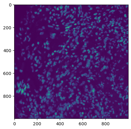
[5]:

plt.imshow(img[:, :, 7])

[5]:

<matplotlib.image.AxesImage at 0x7fe4506fce50>

../_images/examples_link_multiplex_if_8_1.png

[6]:

def plot(slidedata, tile, channel1, channel2):
    image = np.expand_dims(slidedata.tiles[tile].image, axis=0)
    nuc_segmentation_predictions = np.expand_dims(
        slidedata.tiles[tile].masks["nuclear_segmentation"], axis=0
    )
    cell_segmentation_predictions = np.expand_dims(
        slidedata.tiles[tile].masks["cell_segmentation"], axis=0
    )
    # nuc_cytoplasm = np.expand_dims(np.concatenate((image[:,:,:,channel1,0], image[:,:,:,channel2,0]), axis=2), axis=0)
    nuc_cytoplasm = np.stack(
        (image[:, :, :, channel1], image[:, :, :, channel2]), axis=-1
    )
    rgb_images = create_rgb_image(nuc_cytoplasm, channel_colors=["blue", "green"])
    overlay_nuc = make_outline_overlay(
        rgb_data=rgb_images, predictions=nuc_segmentation_predictions.astype("uint8")
    )
    overlay_cell = make_outline_overlay(
        rgb_data=rgb_images, predictions=cell_segmentation_predictions.astype("uint8")
    )
    fig, ax = plt.subplots(1, 2, figsize=(15, 15))
    ax[0].imshow(rgb_images[0, ...])
    ax[1].imshow(overlay_cell[0, ...])
    ax[0].set_title("Raw data")
    ax[1].set_title("Cell Predictions")
    plt.show()

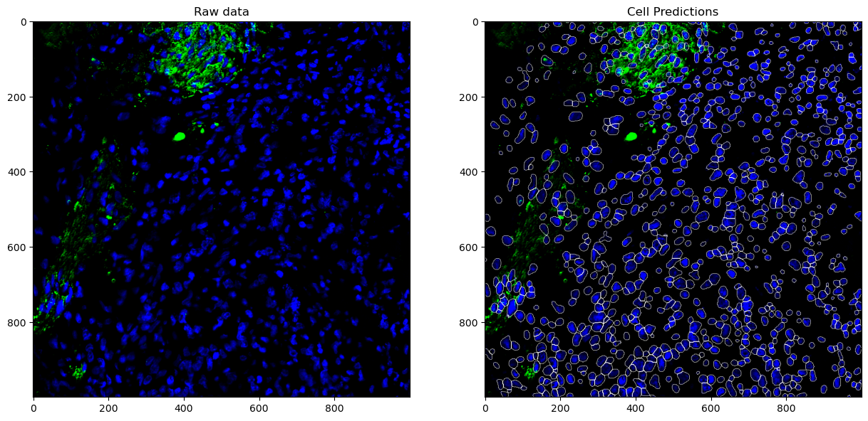
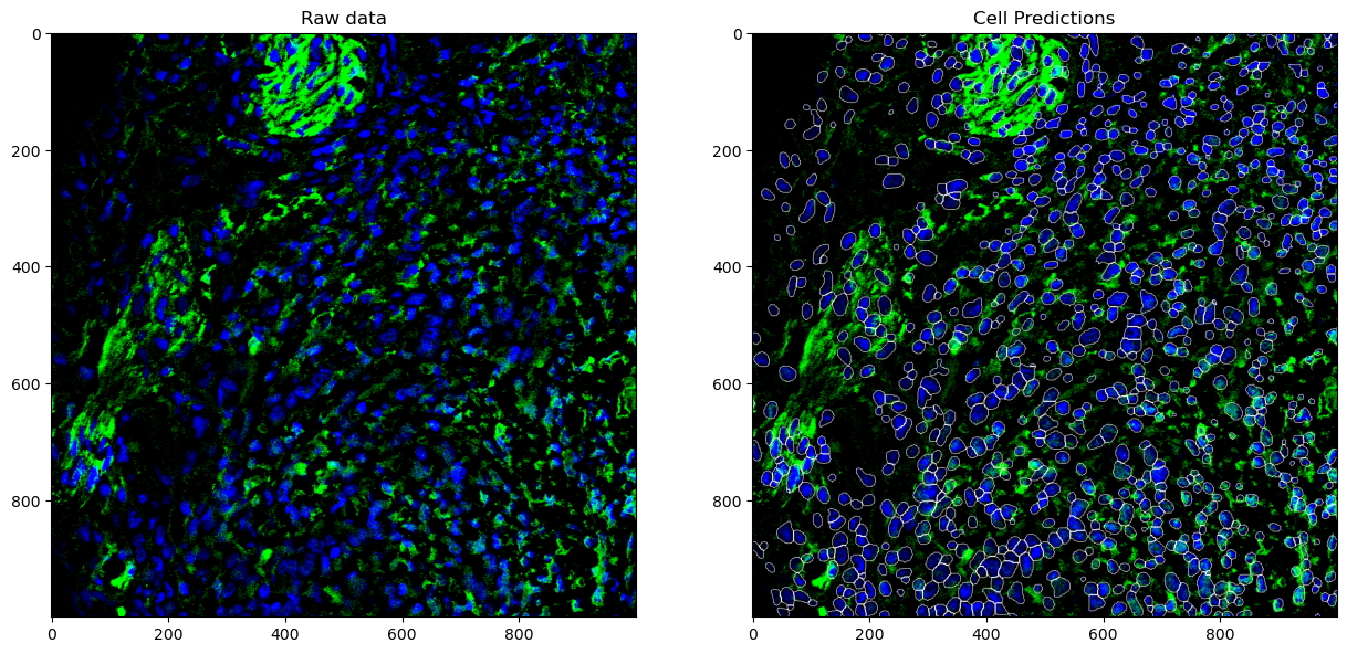
Let’s check the quality of our segmentations in a 1000x1000 pixel tile by looking at DAPI, Syp, and CD44.

[7]:

# DAPI + Syp
plot(slidedata, tile=0, channel1=0, channel2=60)

# DAPI + CD44
plot(slidedata, tile=0, channel1=0, channel2=24)

../_images/examples_link_multiplex_if_11_0.png

../_images/examples_link_multiplex_if_11_1.png

AnnData Integration and Spatial Single Cell Analysis

Now let’s explore the single-cell quantification of our imaging data. Our pipeline produced a single-cell matrix of shape (cell x protein) where each cell has attached additional information including location on the slide and the size of the cell in the image. This information is stored in slidedata.counts as an anndata object (https://anndata.readthedocs.io/en/latest/anndata.AnnData.html).

[8]:

adata = slidedata.counts.to_memory()

[9]:

adata

[9]:

AnnData object with n_obs × n_vars = 945 × 92
    obs: 'y', 'x', 'label', 'filled_area', 'euler_number'
    obsm: 'spatial'
    layers: 'min_intensity', 'max_intensity'

[10]:

adata.X

[10]:

array([[ 8.11290323, 10.98387097, 11.72580645, ...,  0.        ,
         0.        , 21.77419355],
       [10.15277778, 10.90277778, 11.33333333, ...,  0.        ,
         0.        , 23.61111111],
       [20.5       , 17.19642857, 18.51785714, ...,  0.        ,
         0.        , 24.25      ],
       ...,
       [ 9.68345324, 12.20143885, 12.55395683, ...,  0.        ,
         0.        , 12.07913669],
       [ 4.31666667,  8.48333333,  8.65      , ...,  0.        ,
         0.        ,  7.31666667],
       [10.06896552,  8.89655172,  8.79310345, ...,  0.        ,
         0.        ,  8.55172414]])

[11]:

adata.obs

[11]:

	y	x	label	filled_area	euler_number
0	2.048387	219.290323	1	62.0	1
1	2.666667	291.402778	2	72.0	1
2	2.535714	873.107143	3	56.0	1
3	3.729885	550.339080	4	174.0	1
4	3.242105	853.084211	5	95.0	1
...	...	...	...	...	...
940	994.813853	842.056277	941	231.0	1
941	995.741935	336.379032	942	124.0	1
942	995.589928	812.503597	943	139.0	1
943	997.083333	444.583333	944	60.0	1
944	997.517241	966.482759	945	29.0	1

945 rows × 5 columns

[12]:

adata.var

[12]:


0
1
2
3
4
...
87
88
89
90
91

92 rows × 0 columns

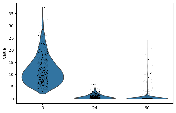
This anndata object gives us access to the entire python (or Seurat) single cell analysis ecosystem of tools. We follow a single cell analysis workflow described in https://scanpy-tutorials.readthedocs.io/en/latest/pbmc3k.html and https://www.embopress.org/doi/full/10.15252/msb.20188746.

[13]:

import scanpy as sc

sc.pl.violin(adata, keys=["0", "24", "60"])
sc.pp.log1p(adata)
sc.pp.scale(adata, max_value=10)
sc.tl.pca(adata, svd_solver="arpack")
sc.pp.neighbors(adata, n_neighbors=10, n_pcs=10)
sc.tl.umap(adata)
sc.pl.umap(adata, color=["0", "24", "60"])

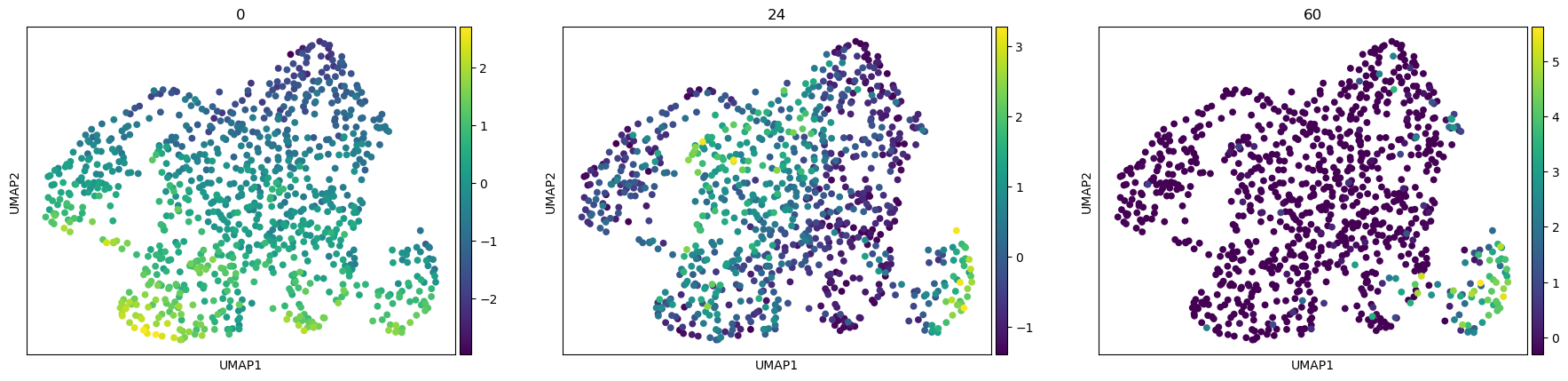
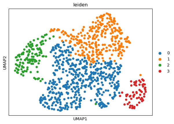
../_images/examples_link_multiplex_if_19_0.png

../_images/examples_link_multiplex_if_19_1.png

[16]:

sc.tl.leiden(adata, resolution=0.15)
sc.pl.umap(adata, color="leiden")
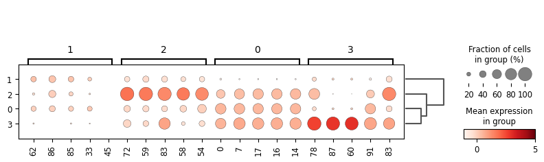
sc.tl.rank_genes_groups(adata, "leiden", method="t-test")
sc.pl.rank_genes_groups_dotplot(adata, groupby="leiden", vmax=5, n_genes=5)

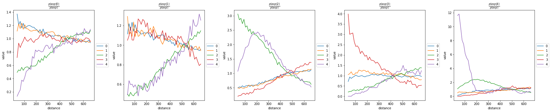
../_images/examples_link_multiplex_if_20_0.png

../_images/examples_link_multiplex_if_20_1.png

We can also use spatial analysis tools such as https://github.com/theislab/squidpy.

[19]:

import scanpy as sc
import squidpy as sq

sc.pl.spatial(adata, color="leiden", spot_size=15)
sc.pl.spatial(adata, color="leiden", groups=["2", "4"], spot_size=15)

[15]:

sq.gr.co_occurrence(adata, cluster_key="leiden")
sq.pl.co_occurrence(adata, cluster_key="leiden")

../_images/examples_link_multiplex_if_23_1.png

References

Schürch, C.M., Bhate, S.S., Barlow, G.L., Phillips, D.J., Noti, L., Zlobec, I., Chu, P., Black, S., Demeter, J., McIlwain, D.R. and Samusik, N., 2020. Coordinated cellular neighborhoods orchestrate antitumoral immunity at the colorectal cancer invasive front. Cell, 182(5), pp.1341-1359.